代码：

# 导入必要的库
import numpy as np
import matplotlib.pyplot as plt

# 定义类1的数据点，每个数据点是二维的坐标
class1_points = np.array([[1.9, 1.2],
                          [1.5, 2.1],
                          [1.9, 0.5],
                          [1.5, 0.9],
                          [0.9, 1.2],
                          [1.1, 1.7],
                          [1.4, 1.1]])

# 定义类2的数据点，每个数据点是二维的坐标
class2_points = np.array([[3.2, 3.2],
                          [3.7, 2.9],
                          [3.2, 2.6],
                          [1.7, 3.3],
                          [3.4, 2.6],
                          [4.1, 2.3],
                          [3.0, 2.9]])

# 将两个类的数据点合并为一个大的数据集 x，标签合并为 y
x = np.concatenate((class1_points, class2_points), axis=0)  # x 是一个 (14, 2) 形状的数组，包含所有的点
y = np.concatenate((np.zeros(len(class1_points)), np.ones(len(class2_points))), axis=0)  # y 是一个包含标签的数组，0 表示 class1，1 表示 class2

# 计算先验概率，即每个类在数据集中的概率
prior_prob = [np.sum(y == 0) / len(y), np.sum(y == 1) / len(y)]

# 计算每个类的均值向量（每个类的特征的均值）
class_u = [np.mean(x[y==0], axis=0), np.mean(x[y==1], axis=0)]

# 计算每个类的协方差矩阵
class_cov = [np.cov(x[y==0], rowvar=False), np.cov(x[y==1], rowvar=False)]

# 定义概率密度函数 (PDF)，用于计算高斯分布的概率
def pdf(x, mean, cov):
    n = len(mean)  # mean 是特征的维度，这里是2，因为每个数据点有两个特征
    # 计算常数系数部分，注意是协方差矩阵的行列式
    coff = 1 / (2 * np.pi) ** (n / 2) * np.sqrt(np.linalg.det(cov))
    # 计算指数部分，(x - mean) 转置和协方差矩阵的逆相乘，再与 (x - mean) 相乘
    exponent = np.exp(-(1 / 2) * np.dot(np.dot((x - mean).T, np.linalg.inv(cov)), (x - mean)))
    # 返回高斯分布的概率密度
    return coff * exponent

# 创建网格点，用于在平面上绘制决策边界
xx, yy = np.meshgrid(np.arange(0, 5, 0.05), np.arange(0, 4, 0.05))

# 将网格点转换为 (N, 2) 的矩阵，方便后续计算
grid_points = np.c_[xx.ravel(), yy.ravel()]

# 用于存储每个网格点的预测标签
grid_label = []

# 遍历网格中的每一个点，计算其后验概率，决定属于哪个类
for point in grid_points:
    poster_prob = []  # 存储每个类的后验概率
    for i in range(2):  # 遍历两个类
        # 计算每个类在该点的似然度（即高斯分布的概率）
        likelihood = pdf(point, class_u[i], class_cov[i])
        # 计算该类的后验概率，即 先验概率 * 似然度
        poster_prob.append(prior_prob[i] * likelihood)
    # 选择后验概率最大的类作为预测的标签
    pre_class = np.argmax(poster_prob)
    grid_label.append(pre_class)

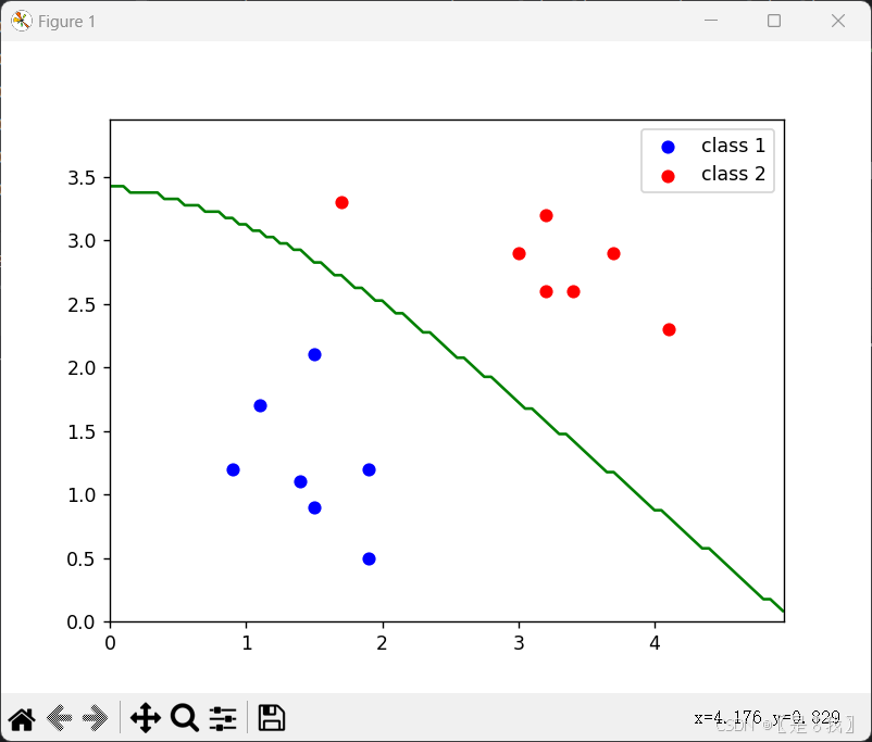
# 绘制类1的样本点，蓝色标记
plt.scatter(class1_points[:, 0], class1_points[:, 1], c='blue', label='class 1')
# 绘制类2的样本点，红色标记
plt.scatter(class2_points[:, 0], class2_points[:, 1], c='red', label='class 2')
# 添加图例
plt.legend()

# 将 grid_label 转换为一个数组，并重塑为与网格形状一致的矩阵，便于绘制等高线图
grid_label = np.array(grid_label)
pre_grid_label = grid_label.reshape(xx.shape)

# 绘制决策边界，等高线图，绿色线表示决策边界（即类0与类1的分界线）
contour = plt.contour(xx, yy, pre_grid_label, levels=[0.5], colors='green')

# 显示绘图结果
plt.show()

结果：